An Introduction to Quotient Space

I’m assuming the reader has some abstract algebra and functional analysis background. You may have learned this already in your linear algebra class, but we are making our way to functional analysis problems.

Motivation

The trouble with $L^p$ spaces

Fix $p$ with $1 \leq p \leq \infty$. It’s easy to see that $L^p(\mu)$ is a topological vector space. But it is not a metric space if we define

$$d(f,g)=\lVert f-g \rVert_p.$$

The reason is, if $d(f,g)=0$, we can only get $f=g$ a.e., but they are not strictly equal. With that being said, this function $d$ is actually a pseudo metric. This is unnatural. However, the relation $\sim$ by $f \sim g \mathbb{R}ightarrow d(f,g)=0$ is a equivalence relation. This inspires us to take the quotient set into consideration.

Vector spaces are groups anyway

For a vector space $V$, every subspace of $V$ is a normal subgroup. There is no reason to prevent ourselves from considering the quotient group and looking for some interesting properties. Further, a vector space is an abelian group, therefore any subspace is automatically normal.

Definition

Let $N$ be a subspace of a vector space $X$. For every $x \in X$, let $\pi(x)$ be the coset of $N$ that contains $x$, that is

$$\pi(x)=x+N.$$

Trivially, $\pi(x)=\pi(y)$ if and only if $x-y \in N$ (say, $\pi$ is well-defined since $N$ is a vector space). This is a linear function since we also have the addition and multiplication by

$$\pi(x)+\pi(y)=\pi(x+y) \quad \alpha\pi(x)=\pi(\alpha{x}).$$

These cosets are the elements of a vector space $X/N$, which reads, the quotient space of $X$ modulo $N$. The map $\pi$ is called the canonical map as we all know.

Examples

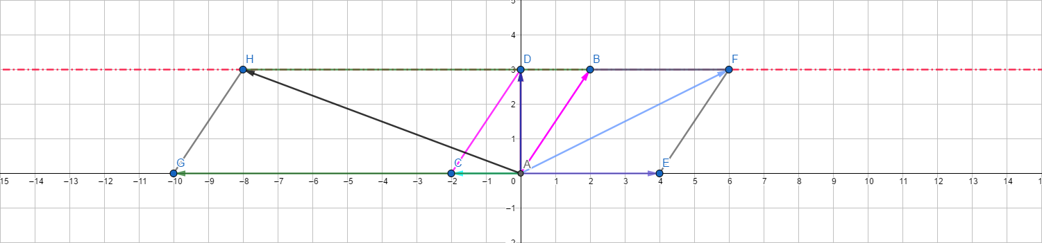
First, we shall treat $\mathbb{R}^2$ as a vector space, and the subspace $\mathbb{R}$, which is graphically represented by $x$-axis, as a subspace (we will write it as $X$). For a vector $v=(2,3)$, which is represented by $AB$, we see the coset $v+X$ has something special. Pick any $u \in X$, for example, $AE$, $AC$, or $AG$. We see $v+u$ has the same $y$ value. The reason is simple since we have $v+u=(2+x,3)$, where the $y$ value remains fixed however $u$ may vary.

With that being said, the set $v+X$, which is not a vector space, can be represented by $\overrightarrow{AD}$. This proceed can be generalized to $\mathbb{R}^n$ with $\mathbb{R}^m$ as a subspace with ease.

---

We now consider a fancy example. Consider all rational Cauchy sequences, that is

$$(a_n)=(a_1,a_2,\cdots)$$

where $a_k\in\mathbb{Q}$ for all $k$. In analysis class, we learned two facts.

1. Any Cauchy sequence is bounded.
2. If $(a_n)$ converges, then $(a_n)$ is Cauchy.

However, the reverse of 2 does not hold in $\mathbb{Q}$. For example, if we put $a_k=(1+\frac{1}{k})^k$, we should have the limit to be $e$, but $e \notin \mathbb{Q}$.

If we define the addition and multiplication term by term, namely

$$(a_n)+(b_n)=(a_1+b_1,a_2+b_2,\cdots)$$

and

$$(\alpha a_n)=(\alpha a_1,\alpha a_2,\cdots)$$

where $\alpha \in \mathbb{Q}$, we get a vector space (the verification is easy). The zero vector is defined by

$$(0)=(0,0,\cdots).$$

This vector space is denoted by $\overline{\mathbb{Q}}$. The subspace containing all sequences converges to $0$ will be denoted by $\overline{\mathbb{O}}$. Again, $(a_n)+\overline{\mathbb{O}}=(b_n)+\overline{\mathbb{O}}$ if and only if $(a_n-b_n) \in \overline{\mathbb{O}}$. Using the language of equivalence relation, we also say $(a_n)$ and $(b_n)$ are equivalent if $(a_n-b_n) \in \overline{\mathbb{O}}$. For example, the two following sequences are equivalent:

$$(1,1,1,\cdots,1,\cdots)\quad\quad (0.9,0.99,0.999,\cdots).$$

Actually, we will get $\mathbb{R} \simeq \overline{\mathbb{Q}}/\overline{\mathbb{O}}$ in the end. But to make sure that this quotient space is exactly the one we meet in our analysis class, there are a lot of verifications should be done.

We shall give more definitions for calculation. The multiplication of two Cauchy sequences is defined term by term à la the addition. For $\overline{\mathbb{Q}}/\overline{\mathbb{O}}$ we have

$$((a_n)+\overline{\mathbb{O}})+((b_n)+\overline{\mathbb{O}})=(a_n+b_n) + \overline{\mathbb{O}}$$

and

$$((a_n)+\overline{\mathbb{O}})((b_n)+\overline{\mathbb{O}})=(a_nb_n)+\overline{\mathbb{O}}.$$

As for inequality, a partial order has to be defined. We say $(a_n) > (0)$ if there exists some $N>0$ such that $a_n>0$ for all $n \geq N$. By $(a_n) > (b_n)$ we mean $(a_n-b_n)>(0)$ of course. For cosets, we say $(a_n)+\overline{\mathbb{O}}>\overline{\mathbb{O}}$ if $(x_n) > (0)$ for some $(x_n) \in (a_n)+\overline{\mathbb{O}}$. This is well defined. That is, if $(x_n)>(0)$, then $(y_n)>(0)$ for all $(y_n) \in (a_n)+\overline{\mathbb{O}}$.

With these operations being defined, it can be verified that $\overline{\mathbb{Q}}/\overline{\mathbb{O}}$ has the desired properties, for example, the least-upper-bound property. But this goes too far from the topic, we are not proving it here. If you are interested, you may visit here for more details.

---

Finally, we are trying to make $L^p$ a Banach space. Fix $p$ with $1 \leq p < \infty$. There is a seminorm defined for all Lebesgue measurable functions on $[0,1]$ by

$$p(f)=\lVert f \rVert_p=\left\{\int_{0}^{1}|f(t)|^pdt\right\}^{1/p}$$

$L^p$ is a vector space containing all functions $f$ with $p(f)<\infty$. But it’s not a normed space by $p$, since $p(f)=0$ only implies $f=0$ almost everywhere. However, the set $N$ which contains all functions that equal $0$ is also a vector space. Now consider the quotient space by

$$\tilde{p}(\pi(f))=p(f),$$

where $\pi$ is the canonical map of $L^p$ into $L^p/N$. We shall prove that $\tilde{p}$ is well-defined here. If $\pi(f)=\pi(g)$, we have $f-g \in N$, therefore

$$0=p(f-g)\geq |p(f)-p(g)|,$$

which forces $p(f)=p(g)$. Therefore in this case we also have $\tilde{p}(\pi(f))=\tilde{p}(\pi(g))$. This indeed ensures that $\tilde{p}$ is a norm, and $L^p/N$ a Banach space. There are some topological facts required to prove this, we are going to cover a few of them.

Topology of quotient space

Definition

We know if $X$ is a topological vector space with a topology $\tau$, then the addition and scalar multiplication are continuous. Suppose now $N$ is a closed subspace of $X$. Define $\tau_N$ by

$$\tau_N=\{E \subset X/N:\pi^{-1}(E)\in \tau\}.$$

We are expecting $\tau_N$ to be properly-defined. And fortunately, it is. Some interesting techniques will be used in the following section.

$\tau_N$ is a vector topology

There will be two steps to get this done.

$\tau_N$ is a topology.

It is trivial that $\varnothing$ and $X/N$ are elements of $\tau_N$. Other properties are immediate as well since we have

$$\pi^{-1}(A \cap B) = \pi^{-1}(A) \cap \pi^{-1}(B)$$

and

$$\pi^{-1}(\cup A_\alpha)=\cup\pi^{-1}( A_{\alpha}).$$

That said, if we have $A,B\in \tau_N$, then $A \cap B \in \tau_N$ since $\pi^{-1}(A \cap B)=\pi^{-1}(A) \cap \pi^{-1}(B) \in \tau$.

Similarly, if $A_\alpha \in \tau_N$ for all $\alpha$, we have $\cup A_\alpha \in \tau_N$. Also, by definition of $\tau_N$, $\pi$ is continuous.

$\tau_N$ is a vector topology.

First, we show that a point in $X/N$, which can be written as $\pi(x)$, is closed. Notice that $N$ is assumed to be closed, and

$$\pi^{-1}(\pi(x))=x+N$$

therefore has to be closed.

In fact, $F \subset X/N$ is $\tau_N$-closed if and only if $\pi^{-1}(F)$ is $\tau$-closed. To prove this, one needs to notice that $\pi^{-1}(F^c)=(\pi^{-1}(F))^{c}$.

Suppose $V$ is open, then

$$\pi^{-1}(\pi(V))=N+V$$

is open. By definition of $\tau_N$, we have $\pi(V) \in \tau_N$. Therefore $\pi$ is an open mapping.

If now $W$ is a neighbourhood of $0$ in $X/N$, there exists a neighbourhood $V$ of $0$ in $X$ such that

$$V + V \subset \pi^{-1}(W).$$

Hence $\pi(V)+\pi(V) \subset W$. Since $\pi$ is open, $\pi(V)$ is a neighbourhood of $0$ in $X/N$, this shows that the addition is continuous.

The continuity of scalar multiplication will be shown in a direct way (so can the addition, but the proof above is intended to offer some special technique). We already know, the scalar multiplication on $X$ by

$$\begin{aligned} \varphi:\Phi \times X &\to X \\ (\alpha,x) &\mapsto \alpha{x} \end{aligned}$$

is continuous, where $\Phi$ is the scalar field (usually $\mathbb{R}$ or $\mathbb{C}$. Now the scalar multiplication on $X/N$ is by

$$\begin{aligned} \psi: \Phi \times X/N &\to X/N \\ (\alpha,x+N) &\mapsto \alpha{x}+N. \end{aligned}$$

We see $\psi(\alpha,x+N)=\pi(\varphi(\alpha,x))$. But the composition of two continuous functions is continuous, therefore $\psi$ is continuous.

A commutative diagram by quotient space

We are going to talk about a classic commutative diagram that you already see in algebra class.

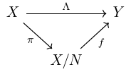
There are some assumptions.

1. $X$ and $Y$ are topological vector spaces.
2. $\Lambda$ is linear.
3. $\pi$ is the canonical map.
4. $N$ is a closed subspace of $X$ and $N \subset \ker\Lambda$.

Algebraically, there exists a unique map $f: X/N \to Y$ by $x+N \mapsto \Lambda(x)$. Namely, the diagram above is commutative. But now we are interested in some analysis facts.

$f$ is linear.

This is obvious. Since $\pi$ is surjective, for $u,v \in X/N$, we are able to find some $x,y \in X$ such that $\pi(x)=u$ and $\pi(y)=v$. Therefore we have

$$\begin{aligned} f(u+v)=f(\pi(x)+\pi(y))&=f(\pi(x+y)) \\ &=\Lambda(x+y) \\ &=\Lambda(x)+\Lambda(y) \\ &= f(\pi(x))+f(\pi(y)) \\ &=f(u)+f(v) \end{aligned}$$

and

$$\begin{aligned} f(\alpha{u})=f(\alpha\pi(x))&=f(\pi(\alpha{x})) \\ &= \Lambda(\alpha{x}) \\ &= \alpha\Lambda(x) \\ &= \alpha{f(\pi(x))} \\ &= \alpha{f(u)}. \end{aligned}$$

$\Lambda$ is open if and only if $f$ is open.

If $f$ is open, then for any open set $U \subset X$, we have

$$\Lambda(U)=f(\pi(U))$$

to be an open set since $\pi$ is open, and $\pi(U)$ is an open set.

If $f$ is not open, then there exists some $V \subset X/N$ such that $f(V)$ is closed. However, since $\pi$ is continuous, we have $\pi^{-1}(V)$ to be open. In this case, we have

$$f(\pi(\pi^{-1}(V)))=f(V)=\Lambda(\pi^{-1}(V))$$

to be closed. $\Lambda$ is therefore not open. This shows that if $\Lambda$ is open, then $f$ is open.

$\Lambda$ is continuous if and only if $f$ is continuous.

If $f$ is continuous, for any open set $W \subset Y$, we have $\pi^{-1}(f^{-1}(W))=\Lambda^{-1}(W)$ to be open. Therefore $\Lambda$ is continuous.

Conversely, if $\Lambda$ is continuous, for any open set $W \subset Y$, we have $\Lambda^{-1}(W)$ to be open. Therefore $f^{-1}(W)=\pi(\Lambda^{-1}(W))$ has to be open since $\pi$ is open.